LAB 7: KALMAN FILTER

Back to Home

The second of a three part sequence culminating in performing stunts with our robot, this lab deals with implementing a Kalman filter using the time-of-flight sensor. The Kalman filter allows us to create a probabilistic estimation of the robot’s state, which can be used to make the PID controller implemented in the previous lab respond quicker depending on data from the ToF sensor.

Collaborators

I worked with Krithik Ranjan and Aryaa Pai for this lab. Due to conducting a last minute fix needed on most of my hardware, I used Krithik’s robot for collecting ToF data and implementing the Kalman filter.

Step Response

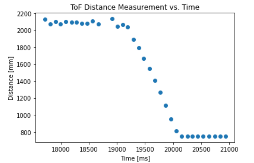
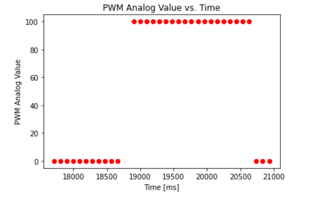
In order to acquire data for the filter, we first need to perform a step response using the robot, which involves driving the robot forward at a constant speed, and stopping it a specific distance before the wall. Since I intended to perform the “Drift Much” stunt with the robot, which involves making the robot drift in a 180 degree turn about 80 centimeters from a wall, my PD controller operated over the gyroscope yaw value and not ToF distance values. Accordingly, I ran the robot at a constant PWM of 100 until it was 80cm away from a wall to obtain relevant data for the filter. Since the ToF sensors are slow and noisy, it was difficult to obtain an exact distance of 80cm - often, I stopped at a distance of roughly 75cm.

Kalman Filter Calculation and Tuning

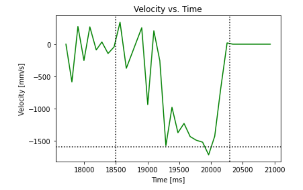
With the measured distance values timestamped, we can roughly compute the velocity profile of the robot as follows (the 90% speed and rise time are annotated on the graph):

Based on the lecture notes, we can compute the A and B matrices as follows:

# Steady state speed = 1.6 m/s ==> d = 1 / 1600 
d = 0.00066

# 90% Rise time = 1.8 ==> m = -d * t_90 / ln(0.1)
m = 4.6903e-04 

A = np.array([  [0,1]   , 
                [0, -d/m]])
B = np.array([  [0] , 
                [1/m]])
                
A = [[1.         0.094     ]
    [0.         0.87975183]]
    
B = [[  0.       ]
    [200.4136196]]
    
C = [[-1, 0]]

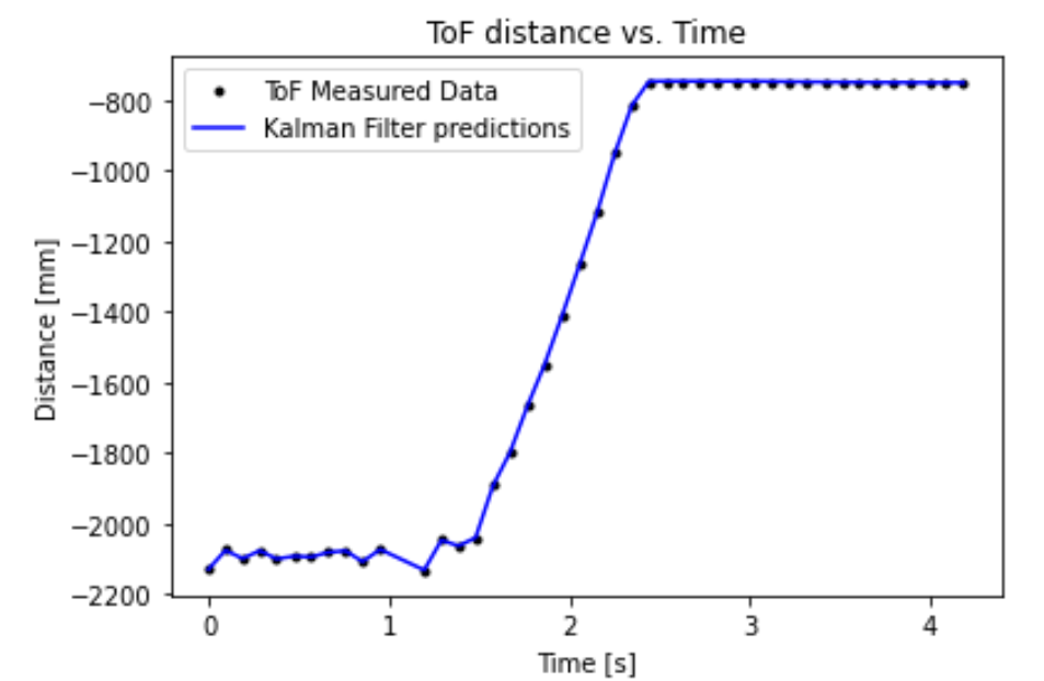
With the A and B matrices calculated, we can use the acquired distance values, the PWM values and the previous state estimation of the robot to calculate the new state as given in the lecture notes. I used the C vector defined for task B in the lecture handout alongside matrices A and B calculated for one timestep; after about 5 iterations, I obtained a fairly precise estimation of the robot’s state using the Kalman filter.

Kalman Filter on the Robot

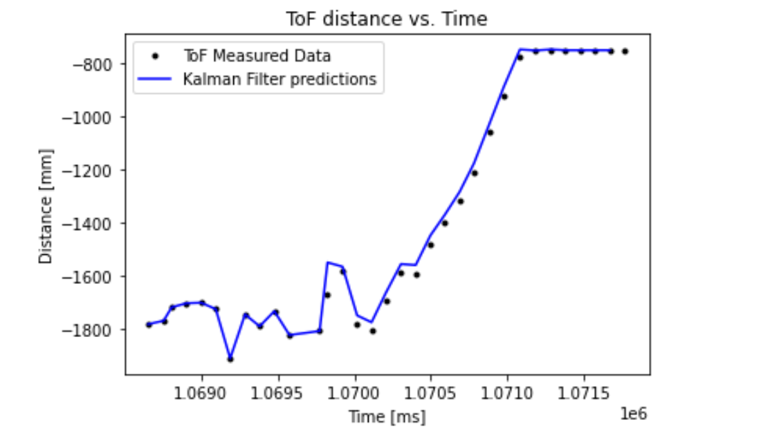
Since the Kalman filter provides a good approximation of the future state of ToF data, it seemed appropriate to use to “speed up” the ToF sensor so that the robot can execute the drift turn at the desired distance in Task B. The method I followed involved recomputing the A and B matrices at every instance of new data, which produces more accurate predictions at the cost of added time complexity. This behavior is not extremely detrimental to the performance of the step response, but could be an issue for the stunt execution (in which case it would be appropriate to use precalculated matrices that do not work as well). We can fix the ranging time of the ToF sensor to get a constant time difference between two consecutive readings, which can be used to compute the A and B state matrices in one iteration of the algorithm (potentially sacrificing some accuracy). The results of the distances obtained from the robot from a drive distance of around 180cm to 80cm and the Kalman filter’s predictions over the data are illustrated below. The filter response seems to fit the data accurately, indicating that I will be able to use it in Lab 8 to speed up the ToF sensor’s sampling time.